Algorithms in Python.
Algorithms as you should know by now are the building blocks of computation. An Algorithm is a detailed sequence of actions to accomplish a specific task. In short an algorithm is a way of producing some output from some input. The context of both the input and output is what defines how a good algorithm computes.
It's important to remember that outside of the theory, an algorithm is represented by the syntax, semantics and constraints of the language you are using to represent it. Thus, the same algorithm will be syntactically different but logically the same in different languages, but here it's all about Python.
Search Algorithms
Search algorithms are widely used to search through data for specific matches. There are many methods for searching data, we will look at a few of the more common methods here.
Searching lists
Binary Search
A binary search is a search on a set of data by way of continuously splitting the data set in half until a match for the required data is found. A divide and conquer approach!
Binary searches are often created as recursive algorithms or functions.
Below is a classic recursive binary search function for a sorted list of integers or strings but not both together.
Note working with numbers is invariably quicker than working with strings in most all search algorithms.
def binary_search(lst, low, high, target):
    """
        A simple recursive binary search algorithm for a sorted list
        Returns index position of target in lst if present, otherwise -1
    """
    # Check base case for the recursive function
    if low <= high:

        mid = (low + high) // 2

        # If Target is  available at the middle itself then return its index
        if lst[mid] == target:
            return mid

        # If the Target is  smaller than mid-value, then search moves
        # left sublist1
        elif lst[mid] > target:
            return binary_search(lst, low, mid - 1, target)

            # Else the search moves to the right sublist1
        else:
            return binary_search(lst, mid + 1, high, target)

    else:
        # Target is  not available in the list1
        return -1
Now, before you say, well that would be easy to do by some simple maths if you have a list of sorted integers from 1 to 100, and you simply use a 0 index math then you don't require a binary search - yes that is correct, why would you? 50 is at index 49 and 1 is at index 0 etc. etc.
But what if the integer values are unknown and not uniform in terms of arithmetic progression, i.e. 1, 2, 4. or 2, 4, 6, 8 ... They may be sorted in order but sorting is not an indication of arithmetic progression. Besides, there are numerous ways to find a position of an item in a data structure in Python, however, the ability to do this via an algorithm without the bells and whistles of Python will enhance your coding skills.
We could also use a simple linear approach with a straight forward iterator, which is fine for small to medium size lists but not when lists get large, very large.
We will see some comparisons later on in the section.
So now we have cleared that up lets continue.
What's going on with this algorithm.
It's fairly straight forward. We pass in the following parameters:
- lst - a list of sorted integers
- low - the initial low index of the list = 0
- high - the len of the list - 1 to compensate for 0 state index
- target - the integer you want to find the position of
In the body of the function we make a quick check to make sure that low index is less than or equal to high index, if low <= high:
We then get the middle point of the list - the middle index. We compare the value at this index with our target, if it matches, the middle point is the position of the target.
If it doesn't match, we compare the value of the middle index value to our target, if it is greater than the target, then this implies that the target is somewhere before the mid-point, the list is sorted remember. In this case we recursively call the function, keeping the low at 0 but setting the high at the mid-point - 1, reducing the computation of the mid-point in the recursive call to the middle of the lower half of the list. If the target i greater than the low middle point value then we set the low value in our recursive call tyo the middle point index + 1. The test for mid-point matching continues in each recursive call until a match ifs found. If eventually low becomes greater than the length of the list then a -1 is returned indicating no match was found.
Let's look at an example:
Example:
target =
15original list =
[1, 2, 3, 4, 5, 12, 15, 19, 20, 30, 37, 42, 53, 55, 101, 128, 132, 189, 201, 300]mid-point-index =
9mid-point-value =
30mid-point-value
30< target =15recursively call the function
new high = mid-point-index - 1 =
8list part to work on next =
[1, 2, 3, 4, 5, 12, 15, 19, 20next mid-point-index =
4mid-point-value =
5< target =15recursively call the function
new low = (mid-point-index + 1) = 5
high remains
8list part to work on next =
12, 15, 19, 20new mid-point-index = '6'
mid-point-value = '15'
return mid-point-index
function recursively unwinds returning the mid-point-index - the value
15is at index6
Note: the list stays complete during the recursive calls it is the low and high values that change the search space of the list.
As mentioned, the above function uses a sorted list. We can sort a list in python by using the sorting method.
Sorting a list
lst = sorted([45,28,9,99,12,43, 21, 1, 5, 7, 99])
str_list = sorted(['one', 'two', 'three', 'four', 'Audi', 'BMW', 'Mercedes', 'Land Rover', 'Toyota', 'Honda'])
will produce
[1, 5, 7, 9, 12, 21, 28, 43, 45, 99, 99]
['Audi', 'BMW', 'Honda', 'Land Rover', 'Mercedes', 'Toyota', 'four', 'one', 'three', 'two']
However, as an example we will use a larger list generated by using the range method to generate a sorted list between 1 and 1000 with increments of 1 which will have be a sorted list anyway, so no need to use the sorted method here.
lst = [*range(1, 1000, 1)]
Next we require the target data that we wish to find.
target = 28
We also need to set the start values of the first and last elements of the list. We will pass these directly to the function when we call it.
result = binary_search(lst, 0, len(lst)-1, target)
We will then print out the result
# Print out the results
if result != -1:
    print("Target is  present at index", str(result))
else:
    print("Target is  not present")
Create a python file and copy the relevant code blocks above in order and run it. With a target of 28
It should return the result as 27 given the target of 28.
It's a straight forward algorithm but with limited usage and several drawbacks. If the list is not sorted, it will return a -1 not found, or if it contains mixed types, say integers and strings, it'll throw an error. Besides, this obvious limitation, this algorithm, written as it is, is quite efficient, so should not be dismissed.
By understanding the way it works you'll get the basics of the binary search.
Now, let's look at a linear search approach vs the binary search, which is both less and more efficient depending on the proximity of the target to either poles of the list and the size of the list as we shall see. In relatively short lists, it is generally more efficient than the binary search function above but much less efficient when the target is further away from the two poles towards the centre ground of a list or the list is large.
Linear Search
Below is a simple linear iterator function
def linear_search(data, target):
    """
        A simple linear search algorithm
        Returns index position of target in data if present, otherwise -1
    """
    # Check base case for the recursive function
    if isinstance(data, list):

        for i in range(len(data)):

            if data[i] == target:
                return i

        # Target was not found
        return -1
The above does the job.
Let's be cleaver and instead of a simple linear iterator let's do it by iterating over a list but from both ends at once. This, is in theory, a binary search as it is searching two different sections of the data object in each iteration. It is searching going forward and going backwards at the same time.
In fact, we covered this form of iteration in the 'Conditions, Loops and Iterators' section of this tutorial.
def linear_search_polar(data, target):
    """
        A simple linear search algorithm that searches from both poles of a list simultaneously
        Returns index position of target in data if present, otherwise -1
    """
    # Check base case for the recursive function
    x = len(data)
    if isinstance(data, list):

        for i in range((len(data) + 1) // 2):

            if data[i] == target:
                return i
            elif data[~i] == target:
                return x - abs(~i)

        # Target was not found
        return -1
Obviously, with both of the above searches you still need to set the data and target. To start, we'll use the same sorted data and target as before.
lst = [*range(1, 1000, 1)]
target = 28

result = binary_search_polar(lst, target)

if result != -1:
    print("Target is  present at index", str(result))
else:
    print("Target is  not present")
Copy the last two linear iterator code blocks and run them. You should get exactly the same result as with the previous function.
Now let's test the speed of the above three functions across a variety of list sizes and targets. To do this we will need to import the inbuilt python library called time and use the perf_counter_ns method to provide time measurements in nanoseconds.
import time

def binary_search(lst, low, high, target):
    """
        A simple recursive binary search algorithm for a sorted list
        Returns index position of target in lst if present, otherwise -1
    """
    # Check base case for the recursive function
    if low <= high:

      mid = (low + high) // 2

      # If Target is  available at the middle itself then return its index
      if lst[mid] == target:
        return mid

      # If the Target is  smaller than mid-value, then search moves
      # left sublist1
      elif lst[mid] > target:
        return binary_search(lst, low, mid - 1, target)

        # Else the search moves to the right sublist1
      else:
        return binary_search(lst, mid + 1, high, target)

    else:
      # Target is  not available in the list1
      return -1

def linear_search(data, target):
    """
        A simple linear search algorithm
        Returns index position of target in data if present, otherwise -1
    """
    # Check base case for the recursive function
    if isinstance(data, list):

        for i in range(len(data)):

            if data[i] == target:
                return i

    # Target was not found
    return -1


def linear_search_polar(data, target):
    """
        A simple linear search algorithm that searches from both poles of a list simultaneously
        Returns index position of target in data if present, otherwise -1
    """
    # Check base case for the recursive function
    x = len(data)
    if isinstance(data, list):

        for i in range((x + 1) // 2):

            if data[i] == target:
                return i
            elif data[~i] == target:
                return x - abs(~i)

      # Target was not found
      return -1

lst = [*range(1, 1000, 1)]
target = 28

tic = time.perf_counter_ns()
result = binary_search(lst, 0, len(lst) - 1, target)
toc = time.perf_counter_ns()
print(f"Binary Search {toc - tic}")

if result != -1:
  print("Target is  present at index", str(result))
else:
  print("Target is  not present")

print("---------------------------------")

tic = time.perf_counter_ns()
result = linear_search(lst, target)
toc = time.perf_counter_ns()
print(f"Linear Search {toc - tic}")

if result != -1:
  print("Target is  present at index", str(result))
else:
  print("Target is  not present")

print("---------------------------------")

tic = time.perf_counter_ns()
result = linear_search_polar(lst, target)
toc = time.perf_counter_ns()
print(f"Linear Search Polar {toc - tic}")

if result != -1:
  print("Target is  present at index", str(result))
else:
  print("Target is  not present")
Copy the code above into a file and run it and see what the times are for each search.
Which was the quickest? On an apple M1 Max pro, the standard linear search is faster, by how much will differ on a case by case basis.
lst = [*range(1, 1000, 1)]
target = 28
---------------------------------
Binary Search 4250
Target is  present at index 27
---------------------------------
Linear Search 2292
Target is  present at index 27
---------------------------------
Linear Search Polar 3167
Target is  present at index 27
Now change the target to 500 and test again.
The results are somewhat different. Our original recursive search seems to be busting it here.
lst = [*range(1, 1000, 1)]
target = 500
---------------------------------
Binary Search 1333
Target is  present at index 499
---------------------------------
Linear Search 13875
Target is  present at index 499
---------------------------------
Linear Search Polar 26833
Target is  present at index 499
Let's change the target to 850 and see what happens
lst = [*range(1, 1000, 1)]
target = 850
---------------------------------
Binary Search 3583
Target is  present at index 849
---------------------------------
Linear Search 23708
Target is  present at index 849
---------------------------------
Linear Search Polar 8958
Target is  present at index 849
As can be seen both the Binary Search and the Linear Search Polar to way better than the straight forward linear search. But the Binary Search is way better than the Linear Search. Obviously rather than linearly iterating through the numbers both the Binary and Polar searches hit the sweet spot by searching at the correct poles of the list first.
Let's push the list up to 100000 and set the target bang smack in the middle at 50000.
lst = [*range(1, 100000, 1)]
target = 50000
---------------------------------
Binary Search 1667
Target is  present at index 49999
---------------------------------
Linear Search 1354417
Target is  present at index 49999
---------------------------------
Linear Search Polar 2675459
Target is  present at index 49999
Now we start to see the difference in extremes. The Binary Search is hitting the sweet spot a lot quicker as it's splitting the list down the middle and 50000 is after all in the middle.
Try larger numbers and different random targets and confirm for yourselves.
Up until now we have been using a sorted list of integers, but what about an unsorted list how do we search that using a Binary Search?
Let's set the list to the following:
lst = random.sample(range(1, 1000), 999)
target = 750
Above we are selecting a random range from 1 to 1000 with 999 numbers.
For this we will need to import the python library random. Add the following import to our test code
import random
Copy the import and the new list and target to your code replacing the old list and target and run the code again.
lst = random.sample(range(1, 1000), 999)
target =750
---------------------------------
Binary Search 4625
Target is  not present
---------------------------------
Linear Search 18375
Target is  present at index 476
---------------------------------
Linear Search Polar 36042
Target is  present at index 476
As you can see the Binary Search cannot cope with unsorted integers as it makes numerical comparisons with mid-points and the target. Given that our numbers are randomly sorted, the target could be anywhere.
But there is a fix. The following function will deal with unsorted lists and mixed lists, i.e. integers, strings, floats whatever. It's not a Binary Search, it simply uses the builtin index method for a list.
Index Search
def index_search(lst, target):
  """
      A simple index search algorithm for an unsorted list
      Returns index position of n in list1 if present, otherwise -1
  """

  # If Target is  available at the middle itself then return its index
  try:
    idx = lst.index(target)
    return idx
  except ValueError as e:
    # Target is  not available in the list1
    return -1
To test this new function copy it to your test code and add a call thus:
tic = time.perf_counter_ns()
result = index_search(lst, target)
toc = time.perf_counter_ns()
print(f"Index Search{toc - tic}")

if result != -1:
    print("Target is  present at index", str(result))
else:
    print("Target is  not present")
Now run the code again
I can't tell you what the result will be as the list we have generated is random so the target could be anywhere in the list. However, you can see the performance is still better than the linear searches.
Try altering the size and target and see what occurs. It still outperforms both linear searches. This is because we have introduced the
list index method into the search. This method directly maps to the list_index_impl C function a for loop in the Cpython. This code uses a C for loop which is of course
ultimately faster than a Python for loop which we have coded in the linear searches.
It's getting interesting now, we are learning about algorithms and their implementation aspects
Let's keep the current set of search functions but switch back to the sorted list. This time let's ramp it right up, say
lst = [*range(1, 10000000, 1)]
target = 80000
Now let's see which is faster.
lst = [*range(1, 10000000, 1)]
target = 80000
---------------------------------
Binary Search 18541
Target is  present at index 79999
---------------------------------
Index Search 486250
Target is  present at index 79999
---------------------------------
Linear Search 2176208
Target is  present at index 79999
---------------------------------
Linear Search Polar 4229666
Target is  present at index 79999
As is clearly seen, the binary search is by far the fastest. This is because we are not iterating over the list with a loop we are using the divide and conquer approach.
Thus far we have discovered that the binary search is pretty much up there when a list is sorted, but gets overtaking by the standard index search when the list is unsorted.
it's swings and roundabouts. Sorting a list takes time too. You could add a timer for checking that yourself.
There is one final twist in this story. The generator.
Index Search using a generator
Look at the following code
def index_search_gen(lst, target):
    """
        A simple index search using a generator
        Returns index position of target in lst if present, otherwise -1
    """
    start = 0
    while True:
        try:
            start = lst.index(target, start)
            yield start
            start += 1
        except ValueError:
            break
We are using a while loop here and a yield statement, and we change the call block slightly to reflect the fact that we are using a generator
tic = time.perf_counter_ns()
result = index_search_gen(lst, target)
toc = time.perf_counter_ns()
print(f"Index Search generator {toc - tic}")
i = str(*result)
if i:
  print("Target is  present at index", i)
else:
  print("Target is  not present")
Notice that the test of the return result looks for the parametrized result as a string which will only have a value if the target is found.
Run this code along with your other search functions and see which comes out on top.
Yeap, the above generator function is way faster than the rest of the functions, but why?
Exercise:
Read up on Python Generators some more and see if you can figure out why it is faster to use the generator with a yield statement in this case rather than a standard return.
Summary
As mentioned previously there are many ways to search through data structures in Python, you may also consider the following:
Converting a list to a dictinary using the
zipfunctionTaking a look at the
bisect_leftmethod from the inbuilt 'bisect' library
It's often useful to optimize search routines but only if it needs optimising. If you only ever have small data structures then it is likely that you will never really need to focus on search optimization, but regardless of this, we have learnt some details regarding Python and the way it works. For those interested in the raw CPython you can find it here:
Algorithms, apart from being an integral part of coding, are useful for learning the intricacies of a programming language and will only serve to enhance your knowledge. Learn as many as possible.
Exercises:
Try writing an efficient mixed type binary search algorithm without using the index function.
Searching Graphs
Searching graphs and matrices is a common task in computer science. There are two classical approaches to this task, depth first search and breath first search.
The semantic difference should be clear. One searches vertically starting, normally, at the first node, whilst the other horizontally, again starting, normally, from the first node.
Both these algorithms when they have reached an end node, i.e. a node with no further connections, backtrack to the previous node and follow that until all nodes have been followed.
In short, it's a process of finding all the paths, i.e. connections between nodes in the graph.
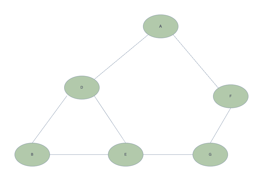
Below is a small graph that we will use to explore both options.
Lets start with the Depth First Search
Depth First Search
The basic depth first search algorithm can be recursive or iterative. Some, such as the following, will return a simple list of nodes in the order they are traversed, whilst others offer a more useful data structure.
Basic depth first search algorithm that returns a list of nodes in the order that they were traversed.
As is depicted below, the graph is a basic Python dictionary. Starting at the root node, we define which nodes from left to right are connected to the root, and then do the same for
each node in each connection adding to the path parameter as we go.
graph = {
  'A' : ['D','F'],
  'D' : ['B', 'E'],
  'B' : ['E'],
  'E' : ['G'],
  'F' : ['G'],
  'G' : []
}

def dfs_recursive(graph, vertex, path=[]):
    """
        Recursively build a path of all the nodes in a graph
    """
    path += [vertex]

    for adjacent in graph[vertex]:

        if adjacent not in path:
            path = dfs_recursive(graph, adjacent, path)

    return path

print(dfs_recursive(graph, 'A'))
The result of running the above function is:
['A', 'D', 'B', 'E', 'G', 'F'].
Let's look at a non-recursive version of the algorithm using a while loop:
graph = {
    'A' : ['D','F'],
    'D' : ['B', 'E'],
    'B' : ['E'],
    'E' : ['G'],
    'F' : ['G'],
    'G' : []
}

def dfs_iterative(graph, start):
    stack, path = [start], []

    while stack:

        vertex = stack.pop()

        if vertex in path:
            continue

        path.append(vertex)

        for adjacent in graph[vertex]:
            stack.append(adjacent)

    return path

print(dfs_iterative(graph, 'A'))
The result of running this function is:
['A', 'F', 'G', 'D', 'E', 'B']
Notice the order is different from the recursive function, but correct nonetheless.
Unlike the recursive version, we're stacking the connections, adjacent nodes, using append method and then popping off the end of the stack, making the order in the resulting list is
from the right to left side of the graph.
Either way, neither function provides us much in terms of branch/route information of the graph. For example, we can't tell from this if B is a node directly connected to A or not and
if D connects to another node or is a terminating node. So unless we know the structure of the graph, which, of course, in this case we do, the resulting lists aren't really a lot of use to us.
Let's remedy this.
We'll start with getting a topology of all the connections between nodes.
graph = {
    'A' : ['D','F'],
    'D' : ['B', 'E'],
    'B' : ['E'],
    'E' : ['G'],
    'F' : ['G'],
    'G' : []
}

def dfs_all_edges_from(graph, vertex, visited, edges=[]):

    visited.append(vertex)

    for vertex in graph[vertex]:
        if vertex not in visited:
            edges = dfs_all_edges_from(graph, vertex, visited.copy(), edges)

    edges.append(visited)
    return edges

print(dfs_all_edges_from(graph, 'A', []))
The above algorithm recursively builds a list of all connections between nodes, the nodes are traversed from left to right, all left side branches in the graph before right side branches. It then backtracks back up to the previous node and looks for any other routes stemming from it. If it finds connecting nodes it traverses those and appends those to the visited list from that node onwards.
Here is the result of running it on our graph.
[['A', 'D', 'B', 'E', 'G'], ['A', 'D', 'B', 'E'], ['A', 'D', 'B'], ['A', 'D', 'E', 'G'], ['A', 'D', 'E'], ['A', 'D'], ['A', 'F', 'G'], ['A', 'F'], ['A']]
The first list ['A', 'D', 'B', 'E', 'G'] represents the edges of all the connecting nodes from the left most branch from the root A to the terminating node G, which has no connecting nodes below it.
After reaching the terminating node, it appends the visited list to edges and returns edges.
It then unwinds the recursion to the previous node in the list, E but there are no more nodes connecting to E in that route, thus it appends the route terminating at E to edges, unwinds the recursion,
backtracking to the previous node in the route B, again no further connecting nodes. Backtracking to D which also connects to E it follows the route from E to the terminating node which is G and adds this route to edges.
resulting in ['A', 'D', 'E', 'G']...
It follows the same pattern across all connecting nodes in each branch stemming from the route node A.
Notice that we are using a copy of
visitedin each recursive call making each visited list independent of the previous.
Now at least we can retrieve a list of all possible branch routes.
Let's take this one step further and find the longest and shortest possible routes between any two nodes in the graph.
The following algorithm takes 6 parameters that are detailed in the doc string of the function
graph = {
    1: [5, 9],
    5: [2, 4],
    9: [8],
    2: [4],
    4: [8],
    8: []
}

def dfs_longest_shortest_routes(graph, vertex, end_node, goal, visited=[], route=None):
    """
        Attempt to find the longest or shortest route between two nodes in a graph.

    :param graph: The graph data structure
    :param vertex: The vertex - the node to start searching from
    :param visited: A list of visited vertexes - initially empty []
    :param end_node: The terminating node to stop searching at
    :param goal: Either min or max for shortest and longest routes specifically. default is min
    :param route: The route matching the goal
    :return:
    """

    visited.append(vertex)

    try:
        for vertex in graph[vertex]:

            if vertex not in visited:

                route = dfs_longest_shortest_routes(graph, vertex, end_node, goal, visited.copy(), route)

                if vertex == end_node:
                    break

        if visited[-1:] == [end_node]:

            if route:
                route = goal(visited, route, key=len)
            else:
                route = visited

    except KeyError:
        pass

    finally:
        return route

print(dfs_longest_shortest_routes(graph, 1, 8, min))
Run the above code and then change the vertex and end_node parameters.
The results will either be the longest or shortest routes or an empty list if invalid vertices or invalid end_node parameters.
As can be seen we have added a try-except block to handle those invalid parameters.
So what is going on with the rest of the algorithm?
- We iterate over the graph.
- If the
vertexhas not beenvisitedwe recursively call the algorithm.- If the
vertexhas beenvisited, and it matches the end_node the break the iteration- If the last item in
visitedmatches theend_nodeassign it toroute.- As part of 4 above, if
routeexists test it against thevisitedparameter with the desiredgoalmin or max. If it doesn't exist a straight assignment is performed.- Return
route- Algorithm unwinds from recursion passing back
routeas it goes.
Notice we use the
finallyin thetry-except-finallyblock to returnroute.finallyis always called regardless of exception status. Also because we have assigned route as an empty list initially if there is an exception then the algorithm returns[]
I think you will agree that this algorithm is of more use than a simple recursive node builder. Now we can identify the longest and shortest path between any two nodes.
But what if we want all routes from a vertex to an end node? We can already get all routes from a vertex using dfs_all_edges_from, but not currently between
two nodes. So let's take a look at that. It's simpler than the previous algorithm so just pick it up and run it.
graph = {
    1: [5, 9],
    5: [2, 4],
    9: [8],
    2: [4],
    4: [8],
    8: []
}

def dfs_all_routes_between_nodes(graph, vertex, end_node, visited=[], routes=[]):
    """
         Attempt to find the longest or shortest route between two nodes in a graph.

     :param graph: The graph data structure
     :param vertex: The vertex - the node to start searching from
     :param visited: A list of visited vertexes - initially empty []
     :param end_node: The terminating node to stop searching at
     :param routes: All the routes that exist between the two nodes
     :return:
     """
    visited.append(vertex)

    try:
        for vertex in graph[vertex]:

            if vertex not in visited:

                routes = dfs_all_routes_between_nodes(graph, vertex, end_node, visited.copy(), routes)

                if vertex == end_node:
                    break

        if visited[-1:] == [end_node]:
            routes.append(visited)

    except KeyError:
        pass

    finally:
        return routes

print(dfs_all_routes_between_nodes(graph, 1, 8))
The result of using the two values 1 and 8 above is:
[[1, 5, 2, 4, 8], [1, 5, 4, 8], [1, 9, 8]]
So now we have a couple of useful algorithms for searching graphs/matrices/tress type structures.
Exercise - Create an algorithm that searches for all routes from a node but upwards.
That's it for this section, you can move on to the next part of this tutorial.